Beta Distribution - Parameter Estimation - Maximum Likelihood - Two Unknown Parameters

Two Unknown Parameters

As it is also the case for maximum likelihood estimates for the gamma distribution, the maximum likelihood estimates for the beta distribution do not have a general closed form solution for arbitrary values of the shape parameters. If are independent random variables each having a beta distribution, the joint log likelihood function for N iid observations is:

$\begin{align} \ln\, \mathcal{L} (\alpha, \beta|X) &= \sum_{i=1}^N \ln\,\mathcal{L}_i (\alpha, \beta|X_i)\\ &= \sum_{i=1}^N \ln\,f(X_i;\alpha,\beta)\\ &= \sum_{i=1}^N \ln\,\frac{\, X_i^{\alpha-1}(1-X_i)^{\beta-1}}{\mathrm{B(\alpha,\beta)}}\\ &= (\alpha - 1)\sum_{i=1}^N \ln X_i + (\beta- 1)\sum_{i=1}^N \ln (1-X_i)-\,N \ln \mathrm{B(\alpha,\beta)} \end{align}$

Finding the maximum with respect to a shape parameter involves taking the partial derivative with respect to the shape parameter and setting the expression equal to zero yielding the maximum likelihood estimator of the shape parameters:

where:

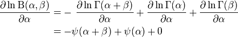
$\begin{align} \frac{\partial \ln \mathrm{B}(\alpha,\beta)}{\partial \alpha} &=-\,\, \frac{\partial \ln \Gamma(\alpha+\beta)}{\partial \alpha}+ \frac{\partial \ln \Gamma(\alpha)}{\partial \alpha}+ \frac{\partial \ln \Gamma(\beta)}{\partial \alpha}\\ &=-\psi(\alpha + \beta) + \psi(\alpha) + 0 \end{align}$

$\begin{align} \frac{\partial \ln \mathrm{B}(\alpha,\beta)}{\partial \beta} &=-\,\, \frac{\partial \ln \Gamma(\alpha+\beta)}{\partial \beta}+ \frac{\partial \ln \Gamma(\alpha)}{\partial \beta}+ \frac{\partial \ln \Gamma(\beta)}{\partial \beta}\\ &=-\psi(\alpha + \beta) + 0 + \psi(\beta) \end{align}$

since the digamma function denoted is defined as the logarithmic derivative of the gamma function:

To ensure that the values with zero tangent slope are indeed a maximum (instead of a saddle-point or a minimum) one has to also satisfy the condition that the curvature is negative. This amounts to satisfying that the second partial derivative with respect to the shape parameters is negative

using the previous equations, this is equivalent to:

where the trigamma function, denoted, is the second of the polygamma functions, and is defined as the derivative of the digamma function: .

These conditions are equivalent to stating that the variances of the logarithmically transformed variables are positive, since:

$\begin{align} \operatorname{var} &= \operatorname{E} - (\operatorname{E})^2 = \psi_1(\alpha) - \psi_1(\alpha + \beta) \end{align}$

$\begin{align} \operatorname{var} &= \operatorname{E} - (\operatorname{E})^2 = \psi_1(\beta) - \psi_1(\alpha + \beta) \end{align}$

Therefore the condition of negative curvature at a maximum is equivalent to the statements:

Alternatively, the condition of negative curvature at a maximum is also equivalent to stating that the following logarithmic derivatives of the geometric means and are positive, since:

(While these slopes are indeed positive: and, the other slopes are negative: and . The slopes of the mean and the median with respect to α and β display similar sign behavior.)

From the condition that at a maximum, the partial derivative with respect to the shape parameter equals zero, we obtain the following system of coupled maximum likelihood estimate equations (for the average log-likelihoods) that needs to be inverted to obtain the (unknown) shape parameter estimates in terms of the (known) average of logarithms of the samples :

where we recognize as the logarithm of the sample geometric mean and as the logarithm of the sample geometric mean based on (1-X), the mirror-image of X. For, it follows that .

These coupled equations containing digamma functions of the shape parameter estimates must be solved by numerical methods as done, for example, by Beckman et al. Gnanadesikan et al. give numerical solutions for a few cases.N.L.Johnson and S.Kotz suggest that for "not too small" shape parameter estimates, the logarithmic approximation to the digamma function may be used to obtain initial values for an iterative solution, since the equations resulting from this approximation can be solved exactly:

which leads to the following solution for the initial values (of the estimate shape parameters in terms of the sample geometric means) for an iterative solution:

Alternatively, the estimates provided by the method of moments can instead be used as initial values for an iterative solution of the maximum likelihood coupled equations in terms of the digamma functions.

When the distribution is required over a known interval other than with random variable X, say with random variable Y, then replace in the first equation with and replace in the second equation with (see "Alternative parametrizations, four parameters" section below).

If one of the shape parameters is known, the problem is considerably simplified. The following logit transformation can be used to solve for the unknown shape parameter (for skewed cases such that, otherwise, if symmetric, both -equal- parameters are known when one is known):

This logit transformation is the logarithm of the transformation that divides the variable X by its mirror-image (X/(1 - X) resulting in the "inverted beta distribution" or beta prime distribution (also known as beta distribution of the second kind or Pearson's Type VI) with support extends the finite support based on the original variable X to infinite support in both directions of the real line .

If, for example, is known, the unknown parameter can be obtained in terms of the inverse digamma function of the right hand side of this equation:

In particular, if one of the shape parameters has a value of unity, for example for (the power function distribution with bounded support ), using the identity in the equation, the maximum likelihood estimator for the unknown parameter is, exactly:

The beta distribution has support, therefore, and hence, and therefore : .

In conclusion, the maximum likelihood estimates of the shape parameters of a beta distribution are (in general) a complicated function of the sample geometric mean, and of the sample geometric mean based on (1-X), the mirror-image of X. One may ask, if the variance (in addition to the mean) is necessary to estimate two shape parameters with the method of moments, why is the (logarithmic or geometric) variance not necessary to estimate two shape parameters with the maximum likelihood method, for which only the geometric means suffice? The answer is because the mean does not provide as much information as the geometric mean. For a beta distribution with equal shape parameters α = β, the mean is exactly 1/2, regardless of the value of the shape parameters, and therefore regardless of the value of the statistical dispersion (the variance). On the other hand, the geometric mean of a beta distribution with equal shape parameters α = β, depends on the value of the shape parameters, and therefore it contains more information. Also, the geometric mean of a beta distribution does not satisfy the symmetry conditions satisfied by the mean, therefore, by employing both the geometric mean based on X and geometric mean based on (1-X), the maximum likelihood method is able to provide best estimates for both parameters α = β, without need of employing the variance.

One can express the joint log likelihood per N iid observations in terms of the sufficient statistics (the sample geometric means) as follows:

We can plot the joint log likelihood per N observations for fixed values of the sample geometric means to see the behavior of the likelihood function as a function of the shape parameters α and β. In such a plot, the shape parameter estimators correspond to the maxima of the likelihood function. See the accompanying graph that shows that all the likelihood functions intersect at α = β = 1, which corresponds to the values of the shape parameters that give the maximum entropy (the maximum entropy occurs for shape parameters equal to unity: the uniform distribution). It is evident from the plot that the likelihood function gives sharp peaks for values of the shape parameter estimators close to zero, but that for values of the shape parameters estimators greater than one, the likelihood function becomes quite flat, with less defined peaks. Obviously, the maximum likelihood parameter estimation method for the beta distribution becomes less acceptable for larger values of the shape parameter estimators, as the uncertainty in the peak definition increases with the value of the shape parameter estimators. One can arrive at the same conclusion by noticing that the expression for the curvature of the likelihood function is in terms of the geometric variances

These variances (and therefore the curvatures) are much larger for small values of the shape parameter α and β. However, for shape parameter values α>1, β>1, the variances (and therefore the curvatures) flatten out. Equivalently, this result follows from the Cramér–Rao bound, since the Fisher information matrix components for the beta distribution are these logarithmic variances. The Cramér–Rao bound states that the variance of any unbiased estimator of is bounded by the reciprocal of the Fisher information:

$\begin{align}\mathrm{var}(\hat{\alpha}) &\geq\frac{1}{\operatorname{var}}\\ &\geq\frac{1}{\psi_1(\hat{\alpha}) - \psi_1(\hat{\alpha} + \hat{\beta})}\\ \end{align}$

$\begin{align}\mathrm{var}(\hat{\beta}) &\geq\frac{1}{\operatorname{var}}\\ &\geq\frac{1}{\psi_1(\hat{\beta}) - \psi_1(\hat{\alpha} + \hat{\beta})}\\ \end{align}$

so the variance of the estimators increases with increasing α and β, as the logarithmic variances decrease.

Also one can express the joint log likelihood per N iid observations in terms of the digamma function expressions for the logarithms of the sample geometric means as follows:

this expression is identical to the negative of the cross-entropy (see section on "Quantities of information (entropy)"). Therefore, finding the maximum of the joint log likelihood of the shape parameters, per N iid observations, is identical to finding the minimum of the cross-entropy for the beta distribution, as a function of the shape parameters.

with the cross-entropy defined as follows:

Read more about this topic: Beta Distribution, Parameter Estimation, Maximum Likelihood

Famous quotes containing the words unknown and/or parameters:

“All nature is but art unknown to thee;
All chance, direction which thou canst not see;
All discord, harmony not understood;
All partial evil, universal good;
And, spite of pride, in erring reason’s spite,
One truth is clear, “Whatever IS, is RIGHT.””
—Alexander Pope (1688–1744)

“What our children have to fear is not the cars on the highways of tomorrow but our own pleasure in calculating the most elegant parameters of their deaths.”
—J.G. (James Graham)

Main Site Subjects